{
"cells": [
{
"cell_type": "markdown",
"metadata": {},
"source": [
"# Linear regression exercises\n",
"\n",
"Credits: Matthew Graham, Pavlos Protopapas\n",
"\n",
"This notebook provides exercises on linear regression. \n",
"\n",
"First we need to do some Python setup."
]
},
{
"cell_type": "code",
"execution_count": null,
"metadata": {
"collapsed": true
},
"outputs": [],
"source": [
"import pandas as pd\n",
"import sys\n",
"import numpy as np\n",
"import scipy as sp\n",
"import matplotlib.pyplot as plt\n",
"import seaborn as sns\n",
"import sklearn as sk\n",
"from sklearn.model_selection import train_test_split\n",
"from sklearn.linear_model import LinearRegression\n",
"sns.set(style=\"ticks\")\n",
"%matplotlib inline"
]
},
{
"cell_type": "markdown",
"metadata": {},
"source": [
"## Load and Explore Data\n",
"\n",
"For these exercises, we're going to use a data set of galaxies with known (spectroscopically confirmed) redshifts and SDSS magnitudes. We're interested in determining the redshift of a galaxy from its colors (photometric redshift).\n",
"First we will load the data and have a look at it. The data can be downloaded from: http://www.astro.caltech.edu/~mjg/sdss_gal.csv.gz\n",
"\n",
"Note that you will need to uncompress the file before using it."
]
},
{
"cell_type": "code",
"execution_count": null,
"metadata": {
"collapsed": true
},
"outputs": [],
"source": [
"sdss_gal_df = pd.read_csv('sdss_gal.csv', low_memory=False)"
]
},
{
"cell_type": "code",
"execution_count": null,
"metadata": {},
"outputs": [],
"source": [
"sdss_gal_df.head()"
]
},
{
"cell_type": "code",
"execution_count": null,
"metadata": {},
"outputs": [],
"source": [
"sdss_gal_df.shape"
]
},
{
"cell_type": "code",
"execution_count": null,
"metadata": {},
"outputs": [],
"source": [
"sdss_gal_df.columns"
]
},
{
"cell_type": "markdown",
"metadata": {},
"source": [
"We'll plot a random subsample of the data to get an idea of what it looks like."
]
},
{
"cell_type": "code",
"execution_count": null,
"metadata": {},
"outputs": [],
"source": [
"sdss_gal_sample = sdss_gal_df.sample(n=1000, random_state=0)\n",
"redshift = sdss_gal_sample['redshift'].values\n",
"gr = sdss_gal_sample['g-r'].values"
]
},
{
"cell_type": "code",
"execution_count": null,
"metadata": {},
"outputs": [],
"source": [
"fig, ax = plt.subplots(1, 1, figsize=(5, 5))\n",
"\n",
"ax.scatter(gr, redshift, color='gray', alpha=0.1)\n",
"\n",
"ax.set_xlabel('g-r')\n",
"ax.set_ylabel('Redshift')\n",
"ax.set_title('SDSS galaxy redshifts:\\n SDSS g-r color vs Redshift Scatter Plot')\n",
"\n",
"plt.show()"
]
},
{
"cell_type": "markdown",
"metadata": {},
"source": [
"---"
]
},
{
"cell_type": "markdown",
"metadata": {},
"source": [
"## The syntax of a regressor\n",
"\n",
"Scikit-learn models have a fixed syntax so it is the same for a simple linear regression operation as it is for something much more complex such as random forest. The specific model is represented as a class with model parameters defined in the class constructor:"
]
},
{
"cell_type": "code",
"execution_count": null,
"metadata": {
"collapsed": true
},
"outputs": [],
"source": [
"class sklearn.linear_model.LinearRegression(\n",
" fit_intercept=True, normalize=False, copy_X=True, n_jobs=1)"
]
},
{
"cell_type": "markdown",
"metadata": {},
"source": [
"The class will also have a fit method for fitting (training) the model which takes the data (X) as a Numpy array of shape [n_samples, n_features] and the response values (y) as a Numpy array of shape [n_samples, n_responses]:"
]
},
{
"cell_type": "code",
"execution_count": null,
"metadata": {
"collapsed": true
},
"outputs": [],
"source": [
"def fit(X, y):\n",
" ..."
]
},
{
"cell_type": "markdown",
"metadata": {},
"source": [
"---"
]
},
{
"cell_type": "markdown",
"metadata": {},
"source": [
"## Modeling the Data\n",
"\n",
"We're going to use train_test_split method to create our training and test data sets for a random subsample. We'll set the test set to be half the size of the training set:"
]
},
{
"cell_type": "code",
"execution_count": null,
"metadata": {
"collapsed": true
},
"outputs": [],
"source": [
"sdss_gal_sample = sdss_gal_df.sample(n=1000, random_state=0)\n",
"\n",
"y = sdss_gal_sample['redshift'].values\n",
"X = sdss_gal_sample['g-r'].values\n",
"\n",
"X_train, X_test, y_train, y_test = train_test_split(X.reshape((len(X), 1)), y, test_size=0.33, random_state=0)"
]
},
{
"cell_type": "markdown",
"metadata": {},
"source": [
"Now we define our basic linear regressor and fit it to the data. You can confirm that the values of the slope and intercept are what you would expect from a MSE loss function."
]
},
{
"cell_type": "code",
"execution_count": null,
"metadata": {},
"outputs": [],
"source": [
"regression = LinearRegression(fit_intercept=True)\n",
"regression.fit(X_train, y_train)\n",
"\n",
"regression_line = lambda x: regression.intercept_ + regression.coef_ * x\n",
"print 'The equation of the regression line is: {} + {} * x'.format(regression.intercept_, regression.coef_[0])"
]
},
{
"cell_type": "markdown",
"metadata": {},
"source": [
"And what does the regression line look like with the data:"
]
},
{
"cell_type": "code",
"execution_count": null,
"metadata": {},
"outputs": [],
"source": [
"fig, ax = plt.subplots(1, 1, figsize=(5, 5))\n",
"\n",
"x_vals = np.linspace(0, 3, 100)\n",
"ax.plot(x_vals, regression_line(x_vals), color='red', linewidth=1.0, label='regression line')\n",
"ax.scatter(X_train, y_train, color='gray', alpha=0.1, label='data')\n",
"\n",
"\n",
"ax.set_xlabel('g-r')\n",
"ax.set_ylabel('Redshift')\n",
"ax.set_title('SDSS Galaxy Redshift Data:\\n Trip Duration vs Fare Scatter Plot')\n",
"ax.legend(loc='best')\n",
"\n",
"plt.show()"
]
},
{
"cell_type": "markdown",
"metadata": {},
"source": [
"---"
]
},
{
"cell_type": "markdown",
"metadata": {},
"source": [
"## Evaluate and Interpret the Model\n",
"\n",
"Let's have a bit more of a look at the linear model we've fitted."
]
},
{
"cell_type": "markdown",
"metadata": {},
"source": [
"### 1. Train vs Test Error\n",
"\n",
"Firstly how the MSE values look for the training and the test data sets:"
]
},
{
"cell_type": "code",
"execution_count": null,
"metadata": {},
"outputs": [],
"source": [
"train_MSE = np.mean((y_train - regression.predict(X_train))**2)\n",
"test_MSE = np.mean((y_test - regression.predict(X_test))**2)\n",
"print 'The train MSE is {}, the test MSE is {}'.format(train_MSE, test_MSE)"
]
},
{
"cell_type": "markdown",
"metadata": {},
"source": [
"### 2. Uncertainty in the Model Parameter Estimates\n",
"\n",
"Now we're going to generate a whole load of random subsamples, fit these, and look at the distributions of the model parameters:"
]
},
{
"cell_type": "code",
"execution_count": null,
"metadata": {
"collapsed": true
},
"outputs": [],
"source": [
"def find_regression_params(regression_model, samples):\n",
" sdss_gal_sample = sdss_gal_df.sample(n=samples)\n",
"\n",
" y = sdss_gal_sample['redshift'].values\n",
" X = sdss_gal_sample['g-r'].values\n",
"\n",
" X_train, X_test, y_train, y_test = train_test_split(X.reshape((len(X), 1)), y, test_size=0.33, random_state=0)\n",
"\n",
" regression_model.fit(X_train, y_train)\n",
" \n",
" return regression_model.intercept_, regression_model.coef_[0]"
]
},
{
"cell_type": "code",
"execution_count": null,
"metadata": {},
"outputs": [],
"source": [
"regression_model = LinearRegression(fit_intercept=True)\n",
"\n",
"total_draws = 500\n",
"samples = 1000\n",
"regression_params = []\n",
"\n",
"for i in range(total_draws):\n",
" if i % 10 == 0:\n",
" out = i * 1. / total_draws * 100\n",
" sys.stdout.write(\"\\r%d%%\" % out)\n",
" sys.stdout.flush()\n",
" \n",
" regression_params.append(find_regression_params(regression_model, samples))\n",
" \n",
"sys.stdout.write(\"\\r%d%%\" % 100)\n",
"regression_params = np.array(regression_params)"
]
},
{
"cell_type": "code",
"execution_count": null,
"metadata": {},
"outputs": [],
"source": [
"fig, ax = plt.subplots(1, 2, figsize=(10, 5))\n",
"\n",
"ax[0].hist(regression_params[:, 0], bins=50, color='blue', edgecolor='white', linewidth=1, alpha=0.2)\n",
"ax[0].axvline(x=regression_params[:, 0].mean(), color='red', label='mean = {0:.2f}'.format(regression_params[:, 0].mean()))\n",
"ax[0].axvline(x=regression_params[:, 0].mean() - 2 * regression_params[:, 0].std(), color='green', linestyle='--', label='std = {0:.2f}'.format(regression_params[:, 0].std()))\n",
"ax[0].axvline(x=regression_params[:, 0].mean() + 2 * regression_params[:, 0].std(), color='green', linestyle='--')\n",
"\n",
"ax[0].set_xlabel('Intercept')\n",
"ax[0].set_ylabel('Frequency')\n",
"ax[0].set_title('Histogram of Estimates of Intercept')\n",
"ax[0].legend(loc='best')\n",
"\n",
"\n",
"ax[1].hist(regression_params[:, 1], bins=50, color='gray', edgecolor='white', linewidth=1, alpha=0.2)\n",
"ax[1].axvline(x=regression_params[:, 1].mean(), color='red', label='mean = {0:.2f}'.format(regression_params[:, 1].mean()))\n",
"ax[1].axvline(x=regression_params[:, 1].mean() - 2 * regression_params[:, 1].std(), color='green', linestyle='--', label='std = {0:.2f}'.format(regression_params[:, 1].std()))\n",
"ax[1].axvline(x=regression_params[:, 1].mean() + 2 * regression_params[:, 1].std(), color='green', linestyle='--')\n",
"\n",
"ax[1].set_xlabel('Slope')\n",
"ax[1].set_ylabel('Frequency')\n",
"ax[1].set_title('Histogram of Estimates of Slope')\n",
"ax[1].legend(loc='best')\n",
"\n",
"plt.tight_layout()\n",
"plt.show()"
]
},
{
"cell_type": "markdown",
"metadata": {},
"source": [
"### 3. The Effect of Sample Size on Uncertainty\n",
"\n",
"We can also look at what the effect of sample size is on the model parameters:"
]
},
{
"cell_type": "code",
"execution_count": null,
"metadata": {},
"outputs": [],
"source": [
"regression_model = LinearRegression(fit_intercept=True)\n",
"\n",
"def compute_SE(total_draws, samples, regression_model):\n",
"\n",
" regression_params = []\n",
"\n",
" for i in range(total_draws):\n",
" regression_params.append(find_regression_params(regression_model, samples))\n",
"\n",
" regression_params = np.array(regression_params)\n",
" return np.std(regression_params[:, 0]), np.std(regression_params[:, 1])\n",
"\n",
"total_draws = 100\n",
"samples = range(100, 10001, 900)\n",
"ses = []\n",
"\n",
"for i in range(len(samples)):\n",
" out = i * 1. / len(samples) * 100\n",
" sys.stdout.write(\"\\r%d%%\" % out)\n",
" sys.stdout.flush()\n",
" ses.append(compute_SE(total_draws, samples[i], regression_model))\n",
"\n",
"sys.stdout.write(\"\\r%d%%\" % 100)"
]
},
{
"cell_type": "code",
"execution_count": null,
"metadata": {},
"outputs": [],
"source": [
"ses = np.array(ses)\n",
" \n",
"fig, ax = plt.subplots(1, 1, figsize=(10, 5))\n",
"\n",
"ax.plot(samples, ses[:, 0], color='teal', label='SE of intercept')\n",
"ax.plot(samples, ses[:, 1], color='brown', label='SE of slope')\n",
"\n",
"ax.set_xlabel('Number of Samples')\n",
"ax.set_ylabel('SE')\n",
"ax.set_title('Uncertainty in Parameter Estimates vs Sample Size')\n",
"ax.legend(loc='best')\n",
"plt.show()"
]
},
{
"cell_type": "markdown",
"metadata": {},
"source": [
"---"
]
},
{
"cell_type": "markdown",
"metadata": {},
"source": [
"## Residual Analysis\n",
"\n",
"In residual analysis we want to check that the residuals are uncorrelated and normally distributed."
]
},
{
"cell_type": "code",
"execution_count": null,
"metadata": {
"collapsed": true
},
"outputs": [],
"source": [
"sdss_gal_df = pd.read_csv('sdss_gal.csv', low_memory=False)"
]
},
{
"cell_type": "code",
"execution_count": null,
"metadata": {},
"outputs": [],
"source": [
"sdss_gal_sample = sdss_gal_df.sample(n=1000, random_state=0)\n",
"\n",
"y = sdss_gal_sample['redshift'].values\n",
"X = sdss_gal_sample['g-r'].values\n",
"\n",
"X_train, X_test, y_train, y_test = train_test_split(X.reshape((len(X), 1)), y, test_size=0.33, random_state=0)\n",
"\n",
"regression = LinearRegression(fit_intercept=True)\n",
"regression.fit(X_train, y_train)\n",
"\n",
"regression_line = lambda x: regression.intercept_ + regression.coef_ * x\n",
"print 'The equation of the regression line is: {} + {} * x'.format(regression.intercept_, regression.coef_[0])"
]
},
{
"cell_type": "markdown",
"metadata": {},
"source": [
"We can also check the value of $R^2$ for both the training and test data sets."
]
},
{
"cell_type": "code",
"execution_count": null,
"metadata": {},
"outputs": [],
"source": [
"train_R_sq = regression.score(X_train, y_train)\n",
"test_R_sq = regression.score(X_test, y_test)\n",
"print 'The train R^2 is {}, the test R^2 is {}'.format(train_R_sq, test_R_sq)"
]
},
{
"cell_type": "code",
"execution_count": null,
"metadata": {},
"outputs": [],
"source": [
"fig, ax = plt.subplots(1, 2, figsize=(10, 5))\n",
"\n",
"errors = y_train - regression.predict(X_train)\n",
"ax[0].scatter(X_train, errors, color='blue', alpha=0.1, label='residuals')\n",
"ax[0].axhline(y=0, color='gold', label='zero error')\n",
"\n",
"\n",
"ax[0].set_xlabel('g-r')\n",
"ax[0].set_ylabel('redshift')\n",
"ax[0].set_title('SDSS Galaxy Redshift Data:\\n Predictor vs Residual')\n",
"ax[0].legend(loc='best')\n",
"\n",
"ax[1].hist(errors, color='blue', alpha=0.1, label='residuals', bins=50, edgecolor='white', linewidth=2)\n",
"ax[1].axvline(x=0, color='gold', label='zero error')\n",
"\n",
"\n",
"ax[1].set_xlabel('g-r')\n",
"ax[1].set_ylabel('redshift')\n",
"ax[1].set_title('SDSS Galaxy Redshift Data:\\n Residual Histogram')\n",
"ax[1].legend(loc='best')\n",
"\n",
"plt.show()"
]
},
{
"cell_type": "markdown",
"metadata": {},
"source": [
"---"
]
},
{
"cell_type": "markdown",
"metadata": {},
"source": [
"## Multiple Linear Regression\n",
"\n",
"Clearly redshift is not just a function of one color but of several so here we will look at fitting a linear model wiht multiple parameters."
]
},
{
"cell_type": "code",
"execution_count": null,
"metadata": {},
"outputs": [],
"source": [
"sdss_gal_sample = sdss_gal_df.sample(n=1000, random_state=0)\n",
"#sdss_gal_sample['lpep_pickup_datetime'] = nyc_cab_sample['lpep_pickup_datetime'].apply(lambda dt: pd.to_datetime(dt).hour)\n",
"#sdss_gal_sample['Lpep_dropoff_datetime'] = nyc_cab_sample['Lpep_dropoff_datetime'].apply(lambda dt: pd.to_datetime(dt).hour)\n",
"msk = np.random.rand(len(sdss_gal_sample)) < 0.8\n",
"train = sdss_gal_sample[msk]\n",
"test = sdss_gal_sample[~msk]\n",
"\n",
"y_train = train['redshift'].values\n",
"X_train = train[['g-r', 'r-i', 'i-z']].values\n",
"\n",
"y_test = test['redshift'].values\n",
"X_test = test[['g-r', 'r-i', 'i-z']].values"
]
},
{
"cell_type": "code",
"execution_count": null,
"metadata": {},
"outputs": [],
"source": [
"multi_regression_model = LinearRegression(fit_intercept=True)\n",
"multi_regression_model.fit(X_train, y_train)\n",
"\n",
"print 'The equation of the regression plane is: {} + {}^T . x'.format(multi_regression_model.intercept_, multi_regression_model.coef_)"
]
},
{
"cell_type": "markdown",
"metadata": {},
"source": [
"### 1. Train vs Test Error\n",
"\n",
"Again we can look at various model diagnostics: first comparing the MSE and $R^2$ values for the training and test data sets:"
]
},
{
"cell_type": "code",
"execution_count": null,
"metadata": {},
"outputs": [],
"source": [
"train_MSE= np.mean((y_train - multi_regression_model.predict(X_train))**2)\n",
"test_MSE= np.mean((y_test - multi_regression_model.predict(X_test))**2)\n",
"print 'The train MSE is {}, the test MSE is {}'.format(train_MSE, test_MSE)\n",
"\n",
"train_R_sq = multi_regression_model.score(X_train, y_train)\n",
"test_R_sq = multi_regression_model.score(X_test, y_test)\n",
"print 'The train R^2 is {}, the test R^2 is {}'.format(train_R_sq, test_R_sq)"
]
},
{
"cell_type": "markdown",
"metadata": {},
"source": [
"### 2. Uncertainty in the Model Parameter Estimates\n",
"\n",
"And the uncertainties in each parameter estimate (u-g, g-r, r-i, i-z):"
]
},
{
"cell_type": "code",
"execution_count": null,
"metadata": {
"collapsed": true
},
"outputs": [],
"source": [
"def find_regression_params(regression_model, samples, cols):\n",
" sdss_gal_sample = sdss_gal_df.sample(n=samples)\n",
"\n",
" y = sdss_gal_sample['redshift'].values\n",
" X = sdss_gal_sample[cols].values\n",
"\n",
" X_train, X_test, y_train, y_test = train_test_split(X, y, test_size=0.33)\n",
"\n",
" regression_model.fit(X_train, y_train)\n",
" \n",
" return np.hstack((np.array([regression_model.intercept_]), regression_model.coef_))\n",
"\n",
"\n",
"def plot_hist_se(vals, bins, title, xlabel, ax):\n",
" mean = vals.mean()\n",
" std = vals.std()\n",
" ax.hist(vals, bins=bins, color='blue', edgecolor='white', linewidth=1, alpha=0.2)\n",
" ax.axvline(mean, color='red', label='mean = {0:.2f}'.format(mean))\n",
" ax.axvline(mean - 2 * std, color='green', linestyle='--', label='std = {0:.2f}'.format(std))\n",
" ax.axvline(mean + 2 * std, color='green', linestyle='--')\n",
"\n",
" ax.set_xlabel(xlabel)\n",
" ax.set_ylabel('Frequency')\n",
" ax.set_title(title)\n",
" ax.legend(loc='best')\n",
"\n",
"\n",
" return ax"
]
},
{
"cell_type": "code",
"execution_count": null,
"metadata": {},
"outputs": [],
"source": [
"total_draws = 500\n",
"samples = 1000\n",
"regression_params = []\n",
"\n",
"for i in range(total_draws):\n",
" if i % 10 == 0:\n",
" out = i * 1. / total_draws * 100\n",
" sys.stdout.write(\"\\r%d%%\" % out)\n",
" sys.stdout.flush()\n",
" \n",
" regression_params.append(find_regression_params(multi_regression_model, samples, ['g-r', 'r-i', 'i-z']))\n",
" \n",
"sys.stdout.write(\"\\r%d%%\" % 100)\n",
"regression_params = np.array(regression_params)"
]
},
{
"cell_type": "code",
"execution_count": null,
"metadata": {},
"outputs": [],
"source": [
"fig, ax = plt.subplots(1, 4, figsize=(20, 5))\n",
"\n",
"ax[0] = plot_hist_se(regression_params[:, 0], 50, 'Histogram of Estimates of Intercept', 'Intercept', ax[0])\n",
"ax[1] = plot_hist_se(regression_params[:, 1], 50, 'Histogram of Estimates of Slope of g-r', 'Slope of g-r', ax[1])\n",
"ax[2] = plot_hist_se(regression_params[:, 2], 50, 'Histogram of Estimates of Slope of r-i', 'Slope of r-i', ax[2])\n",
"ax[3] = plot_hist_se(regression_params[:, 3], 50, 'Histogram of Estimates of Slope of i-z', 'Slope of i-z', ax[3])\n",
"\n",
"plt.tight_layout()\n",
"plt.show()"
]
},
{
"cell_type": "markdown",
"metadata": {},
"source": [
"---"
]
},
{
"cell_type": "markdown",
"metadata": {},
"source": [
"## Evaluating the Significance of Predictors"
]
},
{
"cell_type": "code",
"execution_count": null,
"metadata": {
"collapsed": true
},
"outputs": [],
"source": [
"from statsmodels.tools import add_constant\n",
"\n",
"predictors_multiple = ['g-r', 'r-i', 'i-z']\n",
"predictors_simple = ['g-r']\n",
"\n",
"X_train_multi = add_constant(train[predictors_multiple].values)\n",
"X_test_multi = add_constant(test[predictors_multiple].values)\n",
"\n",
"X_train_simple = add_constant(train[predictors_simple].values)\n",
"X_test_simple = add_constant(test[predictors_simple].values)"
]
},
{
"cell_type": "markdown",
"metadata": {},
"source": [
"### 1. Measuring Significance Using F-Stat, p-Values"
]
},
{
"cell_type": "code",
"execution_count": null,
"metadata": {},
"outputs": [],
"source": [
"import statsmodels.api as sm\n",
"multi_regression_model = sm.OLS(y_train, X_train_multi).fit()\n",
"print 'F-stat:', multi_regression_model.fvalue\n",
"print 'p-values: {} (intercept), {} (g-r), {} (r-i), {} (i-z)'.format(*multi_regression_model.pvalues)"
]
},
{
"cell_type": "markdown",
"metadata": {},
"source": [
"### 2. Measuring Significance Using AIC/BIC"
]
},
{
"cell_type": "code",
"execution_count": null,
"metadata": {},
"outputs": [],
"source": [
"print \"AIC for ['g-r', 'r-i', 'i-z']:\", multi_regression_model.aic\n",
"print \"BIC for ['g-r', 'r-i', 'i-z']:\", multi_regression_model.bic"
]
},
{
"cell_type": "code",
"execution_count": null,
"metadata": {},
"outputs": [],
"source": [
"simple_regression_model = sm.OLS(y_train, X_train_simple).fit()\n",
"print \"AIC for ['g-r']:\", simple_regression_model.aic\n",
"print \"BIC for ['g-r']:\", simple_regression_model.bic"
]
},
{
"cell_type": "markdown",
"metadata": {},
"source": [
"### 3. Measuring Significance Using R^2"
]
},
{
"cell_type": "code",
"execution_count": null,
"metadata": {},
"outputs": [],
"source": [
"simple_model = LinearRegression(fit_intercept=False)\n",
"simple_model.fit(X_train_simple, y_train)\n",
"\n",
"print \"Simple Model: train R^2 = {}, test R^2 = {}\".format(simple_model.score(X_train_simple, y_train), simple_model.score(X_test_simple, y_test))\n",
"\n",
"multiple_model = LinearRegression(fit_intercept=False)\n",
"multiple_model.fit(X_train_multi, y_train)\n",
"\n",
"print \"Multiple Predictor Model: train R^2 = {}, test R^2 = {}\".format(multiple_model.score(X_train_multi, y_train), multiple_model.score(X_test_multi, y_test))"
]
},
{
"cell_type": "markdown",
"metadata": {},
"source": [
"### 4. The Effect of Number of Predictors on R^2"
]
},
{
"cell_type": "code",
"execution_count": null,
"metadata": {
"collapsed": true
},
"outputs": [],
"source": [
"multi_regression_model = LinearRegression(fit_intercept=True)\n",
"\n",
"cols = ['u-g', 'g-r', 'r-i', 'i-z']\n",
"train_R_sq = []\n",
"test_R_sq = []\n",
"for i in range(1, len(cols) + 1):\n",
" predictors = cols[:i]\n",
" X_train = train[predictors].values\n",
" X_test = test[predictors].values\n",
" \n",
" multi_regression_model.fit(X_train, y_train)\n",
" \n",
" train_R_sq.append(multi_regression_model.score(X_train, y_train))\n",
" test_R_sq.append(multi_regression_model.score(X_test, y_test))"
]
},
{
"cell_type": "code",
"execution_count": null,
"metadata": {},
"outputs": [],
"source": [
"fig, ax = plt.subplots(1, 1, figsize=(10, 5))\n",
"\n",
"ax.plot(range(1, len(cols) + 1), train_R_sq, color='blue', label='train R^2')\n",
"ax.plot(range(1, len(cols) + 1), test_R_sq, color='red', label='test R^2')\n",
"\n",
"ax.set_title('Number of Predictor vs Model Fitness')\n",
"ax.set_xlabel('Number of Predictors')\n",
"ax.set_ylabel('R^2')\n",
"ax.legend(loc='best')\n",
"\n",
"plt.show()"
]
},
{
"cell_type": "markdown",
"metadata": {},
"source": [
"---"
]
},
{
"cell_type": "markdown",
"metadata": {},
"source": [
"## Multiple Linear Regression with Interaction Terms\n",
"\n",
"Now we'll consider multiple linear models with cross terms:"
]
},
{
"cell_type": "code",
"execution_count": null,
"metadata": {
"collapsed": true
},
"outputs": [],
"source": [
"from sklearn.preprocessing import PolynomialFeatures\n",
"\n",
"y_train = train['redshift'].values\n",
"X_train = train[['g-r', 'r-i', 'i-z']].values\n",
"\n",
"y_test = test['redshift'].values\n",
"X_test = test[['g-r', 'r-i', 'i-z']].values\n",
"\n",
"gen_cross_terms = PolynomialFeatures(degree=3, interaction_only=True)\n",
"cross_terms = gen_cross_terms.fit_transform(X_train)\n",
"X_train_with_cross = np.hstack((X_train, cross_terms))\n",
"cross_terms = gen_cross_terms.fit_transform(X_test)\n",
"X_test_with_cross = np.hstack((X_test, cross_terms))"
]
},
{
"cell_type": "markdown",
"metadata": {},
"source": [
"Let's get fit statistics for the model with cross terms:"
]
},
{
"cell_type": "code",
"execution_count": null,
"metadata": {},
"outputs": [],
"source": [
"multi_regression_model = LinearRegression(fit_intercept=True)\n",
"multi_regression_model.fit(X_train_with_cross, y_train)\n",
"\n",
"train_MSE = np.mean((y_train - multi_regression_model.predict(X_train_with_cross))**2)\n",
"test_MSE = np.mean((y_test - multi_regression_model.predict(X_test_with_cross))**2)\n",
"print 'The train MSE with interaction terms is {}, the test MSE is {}'.format(train_MSE, test_MSE)\n",
"\n",
"train_R_sq = multi_regression_model.score(X_train_with_cross, y_train)\n",
"test_R_sq = multi_regression_model.score(X_test_with_cross, y_test)\n",
"print 'The train R^2 with interaction terms is {}, the test R^2 is {}'.format(train_R_sq, test_R_sq)"
]
},
{
"cell_type": "markdown",
"metadata": {},
"source": [
"And compare to models without the cross terms:"
]
},
{
"cell_type": "code",
"execution_count": null,
"metadata": {},
"outputs": [],
"source": [
"multi_regression_model.fit(X_train, y_train)\n",
"\n",
"train_MSE = np.mean((y_train - multi_regression_model.predict(X_train))**2)\n",
"test_MSE = np.mean((y_test - multi_regression_model.predict(X_test))**2)\n",
"print 'The train MSE without interaction terms is {}, the test MSE is {}'.format(train_MSE, test_MSE)\n",
"\n",
"train_R_sq = multi_regression_model.score(X_train, y_train)\n",
"test_R_sq = multi_regression_model.score(X_test, y_test)\n",
"print 'The train R^2 without interaction terms is {}, the test R^2 is {}'.format(train_R_sq, test_R_sq)"
]
},
{
"cell_type": "markdown",
"metadata": {},
"source": [
"---"
]
},
{
"cell_type": "markdown",
"metadata": {},
"source": [
"## Polynomial Regression"
]
},
{
"cell_type": "code",
"execution_count": null,
"metadata": {},
"outputs": [],
"source": [
"y_train = train['redshift'].values\n",
"X_train = train[['g-r', 'r-i', 'i-z']].values\n",
"\n",
"y_test = test['redshift'].values\n",
"X_test = test[['g-r', 'r-i', 'i-z']].values\n",
"\n",
"gen_poly_terms = PolynomialFeatures(degree=2, interaction_only=False)\n",
"X_train_with_poly = gen_poly_terms.fit_transform(X_train)\n",
"X_test_with_poly = gen_poly_terms.fit_transform(X_test)"
]
},
{
"cell_type": "code",
"execution_count": null,
"metadata": {},
"outputs": [],
"source": [
"poly_regression_model = LinearRegression(fit_intercept=True)\n",
"poly_regression_model.fit(X_train_with_poly, y_train)\n",
"\n",
"train_MSE= np.mean((y_train - poly_regression_model.predict(X_train_with_poly))**2)\n",
"test_MSE= np.mean((y_test - poly_regression_model.predict(X_test_with_poly))**2)\n",
"print 'The train MSE for degree 2 poly model is {}, the test MSE is {}'.format(train_MSE, test_MSE)\n",
"\n",
"train_R_sq = poly_regression_model.score(X_train_with_poly, y_train)\n",
"test_R_sq = poly_regression_model.score(X_test_with_poly, y_test)\n",
"print 'The train R^2 for degree 2 poly model is {}, the test R^2 is {}'.format(train_R_sq, test_R_sq)"
]
},
{
"cell_type": "markdown",
"metadata": {},
"source": [
"### Effect of Polynomial Degree on Model Performance"
]
},
{
"cell_type": "code",
"execution_count": null,
"metadata": {},
"outputs": [],
"source": [
"from sklearn.preprocessing import MinMaxScaler\n",
"\n",
"train_R_sq = []\n",
"test_R_sq = []\n",
"max_deg = 10\n",
"\n",
"min_max_scaler = MinMaxScaler()\n",
"X_train = min_max_scaler.fit_transform(X_train)\n",
"X_test = min_max_scaler.fit_transform(X_test)\n",
"\n",
"for d in range(max_deg + 1):\n",
"\n",
" out = d * 1. / max_deg * 100\n",
" sys.stdout.write(\"\\r%d%%\" % out)\n",
" sys.stdout.flush()\n",
"\n",
" gen_poly_terms = PolynomialFeatures(degree=d, interaction_only=False)\n",
" X_train_with_poly = gen_poly_terms.fit_transform(X_train)\n",
" X_test_with_poly = gen_poly_terms.fit_transform(X_test)\n",
" \n",
" poly_regression_model = LinearRegression(fit_intercept=False)\n",
" poly_regression_model.fit(X_train_with_poly, y_train)\n",
" \n",
" train_R_sq.append(poly_regression_model.score(X_train_with_poly, y_train))\n",
" test_R_sq.append(poly_regression_model.score(X_test_with_poly, y_test))\n",
" \n",
"sys.stdout.write(\"\\r%d%%\" % 100)"
]
},
{
"cell_type": "code",
"execution_count": null,
"metadata": {},
"outputs": [],
"source": [
"fig, ax = plt.subplots(1, 2, figsize=(15, 5))\n",
"\n",
"ax[0].plot(range(max_deg + 1), np.array(train_R_sq), color='blue', label='train R^2')\n",
"\n",
"ax[0].set_title('Number of Polynomial Degree vs Model Fitness')\n",
"ax[0].set_xlabel('Degree of Polynomial')\n",
"ax[0].set_ylabel('Train R^2')\n",
"ax[0].legend(loc='best')\n",
"\n",
"ax[1].plot(range(max_deg + 1), test_R_sq, color='red', label='test R^2')\n",
"\n",
"ax[1].set_title('Number of Polynomial Degree vs Model Fitness')\n",
"ax[1].set_xlabel('Degree of Polynomial')\n",
"ax[1].set_ylabel('Test R^2')\n",
"ax[1].legend(loc='best')\n",
"\n",
"\n",
"plt.show()"
]
},
{
"cell_type": "markdown",
"metadata": {},
"source": [
"---"
]
},
{
"cell_type": "markdown",
"metadata": {},
"source": [
"## Examples of Overfitting"
]
},
{
"cell_type": "markdown",
"metadata": {},
"source": [
"We're going to overload the train_test_split method to return a number of samples and also a validation set if requested:"
]
},
{
"cell_type": "code",
"execution_count": null,
"metadata": {
"collapsed": true
},
"outputs": [],
"source": [
"sdss_gal_df = pd.read_csv('sdss_gal.csv', low_memory=False)\n",
"\n",
"def train_test_split(df, n_samples, validation=False):\n",
" if validation:\n",
" sdss_gal_sample = df.sample(n=n_samples)\n",
"\n",
" msk = np.random.rand(len(sdss_gal_sample)) < 0.8\n",
" non_test = sdss_gal_sample[msk]\n",
" test = sdss_gal_sample[~msk]\n",
" \n",
" msk = np.random.rand(len(non_test)) < 0.7\n",
" train = non_test[msk]\n",
" validation = non_test[~msk]\n",
" \n",
" return train, validation, test\n",
" \n",
" else:\n",
" sdss_gal_sample = df.sample(n=n_samples)\n",
"\n",
" msk = np.random.rand(len(sdss_gal_sample)) < 0.8\n",
" train = sdss_gal_sample[msk]\n",
" test = sdss_gal_sample[~msk]\n",
"\n",
" return train, test"
]
},
{
"cell_type": "markdown",
"metadata": {},
"source": [
"---"
]
},
{
"cell_type": "markdown",
"metadata": {},
"source": [
"### Too Many Features\n",
"\n",
"The SDSS galaxy redshift data set only has four features but for a higher dimensional data set may be more prone to this effect:"
]
},
{
"cell_type": "code",
"execution_count": null,
"metadata": {},
"outputs": [],
"source": [
"train, test = train_test_split(sdss_gal_df, 50)\n",
"y_train = train['redshift'].values\n",
"y_test = test['redshift'].values\n",
"\n",
"multi_regression_model = LinearRegression(fit_intercept=True)\n",
"\n",
"cols = ['u-g', 'g-r', 'r-i', 'i-z']\n",
"\n",
"train_R_sq = []\n",
"test_R_sq = []\n",
"for i in range(1, len(cols) + 1):\n",
" predictors = cols[:i]\n",
" X_train = train[predictors].values\n",
" X_test = test[predictors].values\n",
" \n",
" multi_regression_model.fit(X_train, y_train)\n",
" \n",
" train_R_sq.append(multi_regression_model.score(X_train, y_train))\n",
" test_R_sq.append(multi_regression_model.score(X_test, y_test))"
]
},
{
"cell_type": "code",
"execution_count": null,
"metadata": {},
"outputs": [],
"source": [
"fig, ax = plt.subplots(1, 1, figsize=(10, 5))\n",
"\n",
"ax.plot(range(1, len(cols) + 1), train_R_sq, color='blue', label='train R^2')\n",
"ax.plot(range(1, len(cols) + 1), test_R_sq, color='red', label='test R^2')\n",
"\n",
"ax.set_title('Number of Predictor vs Model Fitness')\n",
"ax.set_xlabel('Number of Predictors')\n",
"ax.set_ylabel('R^2')\n",
"ax.legend(loc='best')\n",
"\n",
"plt.show()"
]
},
{
"cell_type": "markdown",
"metadata": {},
"source": [
"### Degree Too High\n",
"\n",
"We've already seen this for the polynomial with multiple predictors but we can demonstrate it even with just one predictor:"
]
},
{
"cell_type": "code",
"execution_count": null,
"metadata": {
"collapsed": true
},
"outputs": [],
"source": [
"train, test = train_test_split(sdss_gal_df, 5000)\n",
"y_train = train['redshift'].values\n",
"y_test = test['redshift'].values\n",
"\n",
"poly_regression_model = LinearRegression(fit_intercept=False, normalize=True)\n",
"\n",
"X_train = train[['g-r']].values.reshape((len(train), 1))\n",
"X_test = test[['g-r']].values.reshape((len(test), 1))\n",
"\n",
"train_R_sq = []\n",
"test_R_sq = []\n",
"max_deg = 30\n",
"\n",
"min_max_scaler = MinMaxScaler()\n",
"X_train = min_max_scaler.fit_transform(X_train)\n",
"X_test = min_max_scaler.fit_transform(X_test)\n",
"\n",
"for d in range(1, max_deg):\n",
"\n",
" gen_poly_terms = PolynomialFeatures(degree=d)\n",
" X_train_poly = gen_poly_terms.fit_transform(X_train)\n",
" X_test_poly = gen_poly_terms.fit_transform(X_test)\n",
" \n",
" poly_regression_model.fit(X_train_poly, y_train)\n",
" \n",
" train_R_sq.append(poly_regression_model.score(X_train_poly, y_train))\n",
" test_R_sq.append(poly_regression_model.score(X_test_poly, y_test))\n"
]
},
{
"cell_type": "code",
"execution_count": null,
"metadata": {},
"outputs": [],
"source": [
"fig, ax = plt.subplots(1, 2, figsize=(15, 5))\n",
"\n",
"ax[0].plot(range(1, max_deg), np.array(train_R_sq), color='blue', label='train R^2')\n",
"\n",
"ax[0].set_title('Number of Polynomial Degree vs Model Fitness')\n",
"ax[0].set_xlabel('Degree of Polynomial')\n",
"ax[0].set_ylabel('Train R^2')\n",
"ax[0].legend(loc='best')\n",
"\n",
"ax[1].plot(range(1, max_deg), test_R_sq, color='red', label='test R^2')\n",
"\n",
"ax[1].set_title('Number of Polynomial Degree vs Model Fitness')\n",
"ax[1].set_xlabel('Degree of Polynomial')\n",
"ax[1].set_ylabel('Test R^2')\n",
"ax[1].legend(loc='best')\n",
"\n",
"\n",
"plt.show()"
]
},
{
"cell_type": "markdown",
"metadata": {},
"source": [
"### Parameters are Too Extreme"
]
},
{
"cell_type": "code",
"execution_count": null,
"metadata": {},
"outputs": [],
"source": [
"X_train = np.linspace(0, 40, 20)\n",
"y_train = np.hstack((2 * X_train + 10, np.array([(2 * 45 + 10) * 10000])))\n",
"X_train = np.hstack((X_train, np.array([45])))\n",
"\n",
"regression_model = LinearRegression(fit_intercept=True)\n",
"regression_model.fit(X_train.reshape((len(X_train), 1)), y_train)"
]
},
{
"cell_type": "code",
"execution_count": null,
"metadata": {},
"outputs": [],
"source": [
"fig, ax = plt.subplots(1, 1, figsize=(15, 5))\n",
"\n",
"ax.scatter(X_train, y_train, color='blue', label='data: (x, 2x + 10)')\n",
"ax.plot(X_train, regression_model.intercept_ + regression_model.coef_[0] * X_train, color='red', label='regression line: {}x + {}'.format(regression_model.coef_[0], regression_model.intercept_), )\n",
"\n",
"ax.set_title('Number of Polynomial Degree vs Model Fitness')\n",
"ax.set_xlabel('Degree of Polynomial')\n",
"ax.set_ylabel('Train R^2')\n",
"ax.legend(loc='best')\n",
"plt.show()"
]
},
{
"cell_type": "markdown",
"metadata": {},
"source": [
"---"
]
},
{
"cell_type": "markdown",
"metadata": {},
"source": [
"## Cross Validation For Selecting Polynomial Model Degree\n",
"\n",
"We're going to use k-fold cross validation to determine the degree of the best polynomial for our data:"
]
},
{
"cell_type": "code",
"execution_count": null,
"metadata": {
"collapsed": true
},
"outputs": [],
"source": [
"from sklearn.model_selection import KFold\n",
"\n",
"non_test, test = train_test_split(sdss_gal_df, 5000)\n",
"regression_model = LinearRegression(fit_intercept=False)\n",
"min_max_scaler = MinMaxScaler()\n",
"\n",
"y_non_test = non_test['redshift'].values\n",
"y_test = test['redshift'].values\n",
"\n",
"X_non_test = non_test['g-r'].values.reshape((len(non_test), 1))\n",
"X_test = test['g-r'].values.reshape((len(test), 1))\n",
"\n",
"X_non_test = min_max_scaler.fit_transform(X_non_test)\n",
"X_test = min_max_scaler.fit_transform(X_test)\n",
"\n",
"kf = KFold(n_splits=10)\n",
"\n",
"x_val_scores = []\n",
"\n",
"for d in range(1, 20):\n",
"\n",
" gen_poly_terms = PolynomialFeatures(degree=d, interaction_only=False)\n",
" X_non_test_poly = gen_poly_terms.fit_transform(X_non_test)\n",
"\n",
" validation_R_sqs = []\n",
" for train_index, val_index in kf.split(X_non_test_poly):\n",
" X_train, X_val = X_non_test_poly[train_index], X_non_test_poly[val_index]\n",
" y_train, y_val = y_non_test[train_index], y_non_test[val_index]\n",
"\n",
" regression_model.fit(X_train, y_train)\n",
" validation_R_sqs.append(regression_model.score(X_val, y_val))\n",
" \n",
" x_val_scores.append(np.mean(validation_R_sqs))"
]
},
{
"cell_type": "code",
"execution_count": null,
"metadata": {},
"outputs": [],
"source": [
"fig, ax = plt.subplots(1, 1, figsize=(5, 5))\n",
"\n",
"ax.plot(range(1, 20), x_val_scores, color='blue')\n",
"\n",
"ax.set_title('Polynomial Degree vs Cross Validation Score')\n",
"ax.set_xlabel('Degree of Polynomial')\n",
"ax.set_ylabel('Cross Validation Score')\n",
"\n",
"plt.show()"
]
},
{
"cell_type": "code",
"execution_count": null,
"metadata": {},
"outputs": [],
"source": [
"best_degree = range(1, 20)[np.argmax(x_val_scores)]\n",
"\n",
"gen_poly_terms = PolynomialFeatures(degree=d, interaction_only=False)\n",
"X_non_test_poly = gen_poly_terms.fit_transform(X_non_test)\n",
"X_test_poly = gen_poly_terms.fit_transform(X_test)\n",
"\n",
"regression_model.fit(X_non_test_poly, y_non_test)\n",
"test_R_sq = (regression_model.score(X_test_poly, y_test))\n",
"\n",
"print 'best degree is:', best_degree\n",
"print 'the test R^2 for a degree {} model is: {}'.format(best_degree, test_R_sq)"
]
},
{
"cell_type": "markdown",
"metadata": {},
"source": [
"---"
]
},
{
"cell_type": "markdown",
"metadata": {},
"source": [
"## Comparing Ridge and LASSO Regression"
]
},
{
"cell_type": "code",
"execution_count": null,
"metadata": {
"collapsed": true
},
"outputs": [],
"source": [
"train, validation, test = train_test_split(sdss_gal_df, 5000, validation=True)\n",
"\n",
"y_train = train['redshift'].values\n",
"y_val = validation['redshift'].values\n",
"y_test = test['redshift'].values\n",
"\n",
"regression_model = LinearRegression(fit_intercept=True)\n",
"\n",
"all_predictors = ['u-g', 'g-r', 'r-i', 'i-z']"
]
},
{
"cell_type": "markdown",
"metadata": {},
"source": [
"### 2. Ridge Regression"
]
},
{
"cell_type": "code",
"execution_count": null,
"metadata": {},
"outputs": [],
"source": [
"X_train = train[all_predictors].values\n",
"X_val = validation[all_predictors].values\n",
"X_test = test[all_predictors].values\n",
"\n",
"ridge_regression = Ridge(alpha=1.0, fit_intercept=True)\n",
"ridge_regression.fit(np.vstack((X_train, X_val)), np.hstack((y_train, y_val)))\n",
"\n",
"print 'Ridge regression model:\\n {} + {}^T . x'.format(ridge_regression.intercept_, ridge_regression.coef_)"
]
},
{
"cell_type": "code",
"execution_count": null,
"metadata": {},
"outputs": [],
"source": [
"print 'Train R^2: {}, test R^2: {}'.format(ridge_regression.score(np.vstack((X_train, X_val)), \n",
" np.hstack((y_train, y_val))), \n",
" ridge_regression.score(X_test, y_test))"
]
},
{
"cell_type": "markdown",
"metadata": {},
"source": [
"### 3. LASSO Regression"
]
},
{
"cell_type": "code",
"execution_count": null,
"metadata": {},
"outputs": [],
"source": [
"lasso_regression = Lasso(alpha=1.0, fit_intercept=True)\n",
"lasso_regression.fit(np.vstack((X_train, X_val)), np.hstack((y_train, y_val)))\n",
"\n",
"print 'Lasso regression model:\\n {} + {}^T . x'.format(lasso_regression.intercept_, lasso_regression.coef_)"
]
},
{
"cell_type": "code",
"execution_count": null,
"metadata": {},
"outputs": [],
"source": [
"print 'Train R^2: {}, test R^2: {}'.format(lasso_regression.score(np.vstack((X_train, X_val)), \n",
" np.hstack((y_train, y_val))), \n",
" lasso_regression.score(X_test, y_test))"
]
},
{
"cell_type": "markdown",
"metadata": {},
"source": [
"---"
]
},
{
"cell_type": "markdown",
"metadata": {},
"source": [
"## The Effect of the Regularization Parameter"
]
},
{
"cell_type": "code",
"execution_count": null,
"metadata": {
"collapsed": true
},
"outputs": [],
"source": [
"reg_params = np.hstack((10.**np.arange(-7, 0), 10**np.arange(0, 4) + 0.01))"
]
},
{
"cell_type": "markdown",
"metadata": {},
"source": [
"### 1. Ridge Regression"
]
},
{
"cell_type": "code",
"execution_count": null,
"metadata": {
"collapsed": true
},
"outputs": [],
"source": [
"train_R_sq = []\n",
"test_R_sq = []\n",
"\n",
"for reg in reg_params:\n",
" ridge_regression = Ridge(alpha=reg, fit_intercept=True)\n",
" ridge_regression.fit(np.vstack((X_train, X_val)), np.hstack((y_train, y_val)))\n",
" \n",
" train_R_sq.append(ridge_regression.score(np.vstack((X_train, X_val)), np.hstack((y_train, y_val))))\n",
" test_R_sq.append(ridge_regression.score(X_test, y_test))"
]
},
{
"cell_type": "code",
"execution_count": null,
"metadata": {},
"outputs": [],
"source": [
"fig, ax = plt.subplots(1, 1, figsize=(5, 5))\n",
"\n",
"ax.plot(reg_params, train_R_sq, color='blue', label='train')\n",
"ax.plot(reg_params, test_R_sq, color='red', label='test')\n",
"\n",
"ax.set_xscale('log')\n",
"ax.set_title('Regularization Parameter vs Test R^2')\n",
"ax.set_xlabel('Value of 1/lambda')\n",
"ax.set_ylabel('R^2')\n",
"ax.legend(loc='best')\n",
"\n",
"plt.show()"
]
},
{
"cell_type": "markdown",
"metadata": {},
"source": [
"### 2. LASSO Regression"
]
},
{
"cell_type": "code",
"execution_count": null,
"metadata": {
"collapsed": true
},
"outputs": [],
"source": [
"train_R_sq = []\n",
"test_R_sq = []\n",
"\n",
"for reg in reg_params:\n",
" lasso_regression = Lasso(alpha=reg, fit_intercept=True)\n",
" lasso_regression.fit(np.vstack((X_train, X_val)), np.hstack((y_train, y_val)))\n",
" \n",
" train_R_sq.append(lasso_regression.score(np.vstack((X_train, X_val)), np.hstack((y_train, y_val))))\n",
" test_R_sq.append(lasso_regression.score(X_test, y_test))"
]
},
{
"cell_type": "code",
"execution_count": null,
"metadata": {},
"outputs": [],
"source": [
"fig, ax = plt.subplots(1, 1, figsize=(5, 5))\n",
"\n",
"ax.plot(reg_params, train_R_sq, color='blue', label='train')\n",
"ax.plot(reg_params, test_R_sq, color='red', label='test')\n",
"\n",
"ax.set_xscale('log')\n",
"ax.set_title('Regularization Parameter vs Test R^2')\n",
"ax.set_xlabel('Value of 1/lambda')\n",
"ax.set_ylabel('R^2')\n",
"ax.legend(loc='best')\n",
"\n",
"plt.show()"
]
},
{
"cell_type": "markdown",
"metadata": {},
"source": [
"---"
]
},
{
"cell_type": "markdown",
"metadata": {},
"source": [
"## Cross Validation: Selecting the Regularization Parameter"
]
},
{
"cell_type": "code",
"execution_count": null,
"metadata": {
"collapsed": true
},
"outputs": [],
"source": [
"X_non_test = np.vstack((X_train, X_val))\n",
"y_non_test = np.hstack((y_train, y_val))\n",
"\n",
"\n",
"kf = KFold(n_splits=10)\n",
"\n",
"x_val_scores = []\n",
"\n",
"for reg in reg_params:\n",
" ridge_regression = Ridge(alpha=reg, fit_intercept=True)\n",
" \n",
" validation_R_sqs = []\n",
" for train_index, val_index in kf.split(X_non_test):\n",
" X_train, X_val = X_non_test[train_index], X_non_test[val_index]\n",
" y_train, y_val = y_non_test[train_index], y_non_test[val_index]\n",
"\n",
" \n",
" ridge_regression.fit(X_train, y_train)\n",
" validation_R_sqs.append(ridge_regression.score(X_val, y_val))\n",
" \n",
" x_val_scores.append(np.mean(validation_R_sqs))"
]
},
{
"cell_type": "code",
"execution_count": null,
"metadata": {},
"outputs": [],
"source": [
"fig, ax = plt.subplots(1, 1, figsize=(5, 5))\n",
"\n",
"ax.plot(reg_params, x_val_scores, color='blue')\n",
"\n",
"ax.set_xscale('log')\n",
"ax.set_title('Regularization Strength vs Cross Validation Score')\n",
"ax.set_xlabel('Strength of Regularization')\n",
"ax.set_ylabel('Cross Validation Score')\n",
"\n",
"plt.show()"
]
},
{
"cell_type": "code",
"execution_count": null,
"metadata": {},
"outputs": [],
"source": [
"best_alpha = reg_params[np.argmax(x_val_scores)]\n",
"\n",
"ridge_regression = Ridge(alpha=best_alpha, fit_intercept=True)\n",
"ridge_regression.fit(X_non_test, y_non_test)\n",
"test_R_sq = (ridge_regression.score(X_test, y_test))\n",
"\n",
"print 'best regularization param is:', best_alpha\n",
"print 'the test R^2 for ridge regression with alpha = {} is: {}'.format(best_alpha, test_R_sq)"
]
},
{
"cell_type": "markdown",
"metadata": {},
"source": [
"---"
]
},
{
"cell_type": "markdown",
"metadata": {},
"source": [
"## Bias-Variance Tradeoff"
]
},
{
"cell_type": "markdown",
"metadata": {},
"source": [
"Consider a regression model that fits perfectly the *training data* (e.g. high order polynomial or small $h$). This complex model will have a high variance when regressing new data. On the other hand, a model too simple will have very low variance, but at the same time it will have a high bias. Furthermore, there is a tradeoff between bias and variance in terms of the MSE of the model:\n",
"\n",
"$\\mathrm{MSE}(x) = \\mathbb{E}(f(x) - \\hat{f}(x)) = \\mathrm{bias}_x^2 + \\mathrm{variance}_x + \\sigma^2$, where\n",
"\n",
"$\\mathrm{bias}_x = \\mathbb{E}(\\hat{f}(x))- f(x)$\n",
"\n",
"$\\mathrm{variance}_x = \\mathrm{Var}(\\hat{f}(x)) = \\mathbb{E}(\\hat{f}(x) - \\mathbb{E}(\\hat{f}(x)))$\n",
"\n",
"$\\sigma$ = standard deviation of the noise.\n",
"\n",
"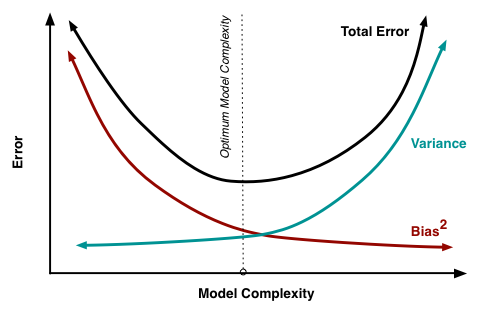 \n"
]
},
{
"cell_type": "code",
"execution_count": null,
"metadata": {},
"outputs": [],
"source": [
"x = np.arange(0, 2*np.pi, 0.01)\n",
"y = np.cos(2*x)\n",
"\n",
"sigma_noise = 0.1\n",
"N = 5\n",
"pl.clf()\n",
"\n",
"pl.plot(x, y, \"k\")\n",
"colors = ['r', 'b', 'g', 'c', \"m\", \"y\"]\n",
"for i in range(N):\n",
" x_data = np.random.random(10)*2*np.pi\n",
" y_data = np.cos(2*x_data) + np.random.normal(scale = sigma_noise, size = 10)\n",
"\n",
" p1 = np.polyfit(x_data, y_data, 0)\n",
" p1 = np.poly1d (p1)\n",
" y1 = p1(x)\n",
"\n",
" pl.plot(x_data, y_data, \"o\" + colors[i])\n",
" pl.plot (x, y1, colors[i])\n",
"pl.title (\"0 order poly: high bias, low variance\")\n",
"pl.ylim ([-3, 3]) \n",
"pl.show()\n",
"\n",
"pl.clf()\n",
"pl.plot(x, y, \"k\")\n",
"for i in range(N):\n",
" x_data = np.random.random(10)*2*np.pi\n",
" y_data = np.cos(2*x_data) + np.random.normal(scale = sigma_noise, size = 10)\n",
"\n",
" p10 = np.polyfit(x_data, y_data, 8)\n",
" p10 = np.poly1d (p10)\n",
" y10 = p10(x)\n",
"\n",
" pl.plot(x_data, y_data, \"o\" + colors[i])\n",
" pl.plot (x, y10, colors[i])\n",
"pl.title (\"9th order poly: low bias, high variance\")\n",
"pl.ylim ([-3, 3])\n",
"pl.show()"
]
},
{
"cell_type": "markdown",
"metadata": {},
"source": [
"In general, the more biased our model is, the lowest the variance, and vice versa. The good news is that we can balance variance and bias using the RMSE over a _test set_. This is the same concept of cross-validation used in classification.\n",
"\n"
]
}
],
"metadata": {
"anaconda-cloud": {},
"kernelspec": {
"display_name": "Python 2",
"language": "python",
"name": "python2"
},
"language_info": {
"codemirror_mode": {
"name": "ipython",
"version": 2
},
"file_extension": ".py",
"mimetype": "text/x-python",
"name": "python",
"nbconvert_exporter": "python",
"pygments_lexer": "ipython2",
"version": "2.7.13"
},
"name": "_merged"
},
"nbformat": 4,
"nbformat_minor": 1
}
\n"
]
},
{
"cell_type": "code",
"execution_count": null,
"metadata": {},
"outputs": [],
"source": [
"x = np.arange(0, 2*np.pi, 0.01)\n",
"y = np.cos(2*x)\n",
"\n",
"sigma_noise = 0.1\n",
"N = 5\n",
"pl.clf()\n",
"\n",
"pl.plot(x, y, \"k\")\n",
"colors = ['r', 'b', 'g', 'c', \"m\", \"y\"]\n",
"for i in range(N):\n",
" x_data = np.random.random(10)*2*np.pi\n",
" y_data = np.cos(2*x_data) + np.random.normal(scale = sigma_noise, size = 10)\n",
"\n",
" p1 = np.polyfit(x_data, y_data, 0)\n",
" p1 = np.poly1d (p1)\n",
" y1 = p1(x)\n",
"\n",
" pl.plot(x_data, y_data, \"o\" + colors[i])\n",
" pl.plot (x, y1, colors[i])\n",
"pl.title (\"0 order poly: high bias, low variance\")\n",
"pl.ylim ([-3, 3]) \n",
"pl.show()\n",
"\n",
"pl.clf()\n",
"pl.plot(x, y, \"k\")\n",
"for i in range(N):\n",
" x_data = np.random.random(10)*2*np.pi\n",
" y_data = np.cos(2*x_data) + np.random.normal(scale = sigma_noise, size = 10)\n",
"\n",
" p10 = np.polyfit(x_data, y_data, 8)\n",
" p10 = np.poly1d (p10)\n",
" y10 = p10(x)\n",
"\n",
" pl.plot(x_data, y_data, \"o\" + colors[i])\n",
" pl.plot (x, y10, colors[i])\n",
"pl.title (\"9th order poly: low bias, high variance\")\n",
"pl.ylim ([-3, 3])\n",
"pl.show()"
]
},
{
"cell_type": "markdown",
"metadata": {},
"source": [
"In general, the more biased our model is, the lowest the variance, and vice versa. The good news is that we can balance variance and bias using the RMSE over a _test set_. This is the same concept of cross-validation used in classification.\n",
"\n"
]
}
],
"metadata": {
"anaconda-cloud": {},
"kernelspec": {
"display_name": "Python 2",
"language": "python",
"name": "python2"
},
"language_info": {
"codemirror_mode": {
"name": "ipython",
"version": 2
},
"file_extension": ".py",
"mimetype": "text/x-python",
"name": "python",
"nbconvert_exporter": "python",
"pygments_lexer": "ipython2",
"version": "2.7.13"
},
"name": "_merged"
},
"nbformat": 4,
"nbformat_minor": 1
}